
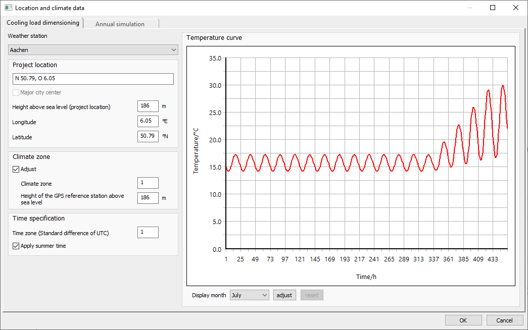

The cooling load calculation according to VDI 2078 is based on a defined heat period of 19 days with increasing temperatures up to the maximum design temperature on the actual design day, the CDD (Cooling Design Day). The annual simulation, on the other hand, uses realistic weather patterns of a whole year for calculation, i.e. the hour-based test reference year data (TRY) of the German Meteorological Service (Deutscher Wetterdienst). The weather data from the TRY differ significantly from the solar radiation values and outdoor temperatures during the defined heat periods of the cooling load calculation (see Fig. 1a and 1b). Due to the different basic conditions, the results of the highest cooling load differ between the cooling load calculation and the annual simulation. In addition to the highest cooling load, the annual simulation can be used to calculate the annual energy demand for heating and cooling, as well as the highest heating and cooling load and its timing. Furthermore the annual simulation provides the operating hours of the heating and cooling system for the entire building or individual rooms.
Among other things, the results of the annual simulation can be used to design heating and cooling systems with the highest possible base load and the lowest possible peak load. This additional information from the annual simulation is available without additional effort, since both calculations are performed with the same settings for internal loads and temperature profiles.
Sample project
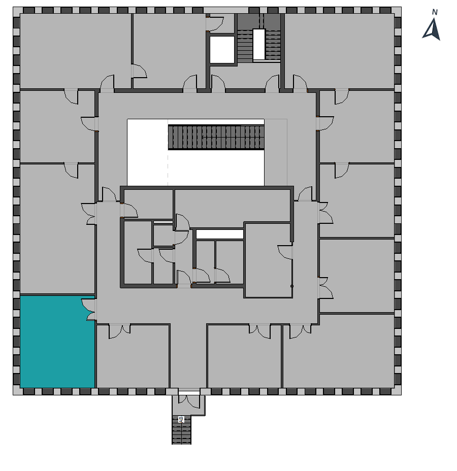
With help of a sample project, the differences between the results from the annual simulation and the dynamic cooling load calculation are to be clarified. For comparison, a corner room on the second floor with south-west orientation is examined (see Fig. 2). The building is located in Aachen, Germany and the internal loads correspond to the values from the previous parts of the article series and remain unchanged. In this article, the factors of operation, control concept and weather data are considered as variable parameters. Cooling load calculations are repeatedly performed with varying parameters and their influence on the results is discussed.
Influence of the operating time of the cooling system
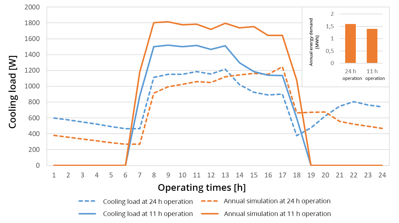
When observing the influence of operating times, a continuous operating time of the cooling system (24 h operation on 7 days per week) is compared with a reduced operating time (11 h operation on the 5 working days). A cooling load calculation and annual simulation are performed for both operating periods. The curves on the design day of the cooling load calculation and the day with the highest cooling capacity from the annual simulation are shown in Fig. 3. In addition, the annual cooling energy demand of the two annual simulations is provided here. The maximum required cooling capacity is indicated for the “11h operation”. This behavior is mainly due to the storage capacity of the components. In “24h operation”, the solar heat stored during the day is discharged via the cooling system at night. - In "11h operation", the temperature of the components is higher at the beginning of the operating time and the components can store less heat during the day, which leads to a higher cooling capacity. If, in parallel to the maximum cooling capacity, the annual cooling energy demand from the annual simulation is considered, it becomes clear, although the “11h operation” results in higher maximum cooling loads, the annual energy demand is lower than for the "24h operation". Thus, the operating time of the cooling system not only influences the cooling load, but also the annual energy demand. Extending the operating time lowers the required maximum cooling capacity and the cooling energy demand increases. This effect increases with increasing effective heat storage capacity.

Influence of the control concept
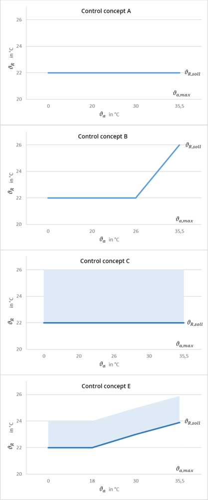
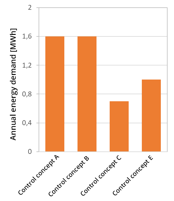
VDI 2078 describes various control concepts for the operation of the cooling system. There are control concepts with constant or outside temperature-controlled room temperatures. Furthermore, there are control concepts with a temperature band, where a 2-point or proportional control can be used. The extent of the influence of the control concepts on the required cooling capacity and cooling energy demand is illustrated below using four control concepts. For this purpose, the maximum values from cooling load calculation and annual simulation are calculated for the corner room at "24h operation". Fig. 4 shows the target temperatures of the control concepts. Control concept A regulates the room to a constant room temperature of 22 °C. With this control concept, the room is cooled as soon as the room temperature rises without cooling, i.e. when more energy is supplied to the room than it can dissipate. To ensure that the room temperature is always kept constant, the room is also heated immediately if less energy is supplied to the room than it dissipates via the external surfaces. Also, for control concept B, a constant room temperature is used. In this case, the room temperature is linked to the outside temperature. Up to an outside temperature of 26 °C, a room temperature of 22 °C is applied, just as in control concept B. At higher outside temperatures the room temperature is increased linearly up to 26 °C. The control concepts C and E are 2-point controls. In 2-point controls a temperature range is defined, in which the room temperature is allowed to fluctuate. The temperature band is defined by a minimum and maximum room temperature. Cooling starts when the room temperature rises above the maximum temperature. In control concept C the minimum room temperature is set at 22 °C and has a temperature band of 4 K, so that the room is cooled from a room temperature of 26 °C. - As with control concept B the minimum room temperature in control concept E is linked to the outside temperature. In contrast to control concept B the room temperature in control concept E already rises at an outside temperature of 18 °C. Since the maximum room temperature is also 26 °C the increase of the room temperature in control concept E is lower than in control concept B. The results of the calculations for the maximum cooling capacity are shown in Fig. 5 and those of the annual cooling energy demand in Fig. 6.
As already shown for the operating times, the maximum cooling capacity in the annual simulation is also slightly higher for the control concepts than for the cooling load calculation. A comparison of the control concepts shows that the highest cooling capacity is required for control concept A. The required capacity is lower with control concepts B and C. The lowest cooling load is reached with control concept E. On the other hand control concept C has the lowest annual energy demand for cooling. The differences between the control concepts are due to the different maximum permitted room temperatures and the differences in the load profiles.
The largest difference between the outside temperature and the room temperature occurs with control concept A. With control concepts B and E, which are based on the outside temperature, the room temperature increases to 26 °C in the afternoon of the design day and is thus higher than with control concept A, which has a constant temperature of 22 °C. Due to the lower room temperature, control concept A requires the highest cooling capacity. The moving room temperature that depends on the outside temperature also influences the load profile of the cooling load. This differs significantly from a load profile with a constant room temperature. To illustrate the difference, the load curves of both 2-point control concepts are compared in Fig. 7. In control concept C (constant room temperature), the cooling load increases during the day and the highest cooling load is reached at 5 pm.
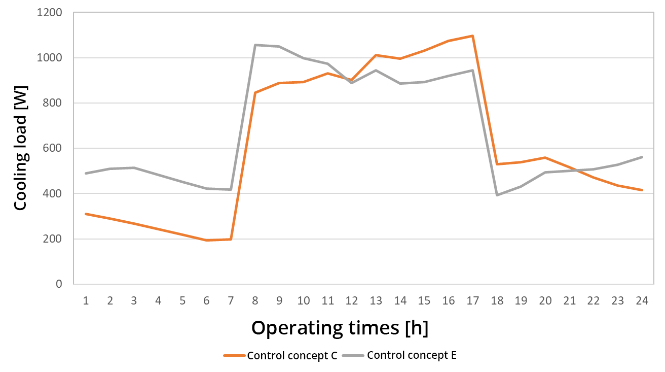
In contrast, the highest cooling load in control concept E (moving room temperature) is already reached at 8 am. Due to the rising outside temperature and the constant indoor temperature, the highest cooling load in the control concepts with constant room temperature is reached in the afternoon, since the outside temperatures are highest at that moment and the walls have heated up during the day. With control concept E on the other hand the room temperature is lowest in the morning, and even before the direct solar radiation reaches the room (windows to south/west orientation), the outdoor temperature rises and thus also the Target room temperature. The increasing target temperature of the room compensates for the increasing solar heat in the room and the cooling load decreases throughout the day. The fact that the maximum cooling load for control concept C with the constant room temperature is higher than for control concept E results from the low wall temperatures. Due to the low target room temperature at night, the walls have a lower temperature in the morning than in control concept C. This can especially be observed in the higher cooling capacity during the night. Due to the lower wall temperatures, the walls are able to absorb more energy during the day and reduce the maximum cooling load. The greater cooling at night also explains why the lowest annual energy demand for cooling is achieved with control concept C: this control concept always uses the highest target room temperature of 26 °C for cooling.
Different test reference years
The test reference years (TRY) used for the calculation of the annual simulation are based on weather data which provided a representative value for each hour of the year. The German Weather Service provides the TRY for all of Germany with a resolution of one square kilometer free of charge. Six different data sets are included for each of these locations. Two reference periods are supplied. The TRY-2015 refer to weather data from 1995 to 2012 and represent the present. The second reference period TRY-2045 represents a future prognosis. This is determined based on weather models and represents the period from year 2031 to 2060. For both reference periods, TRY data is provided for a “Normal Year", an "Extreme Summer" and an "Extreme Winter".The Normal Year of TRY-2015 corresponds to an average of all years of the selected period. For extreme TRY, one year with the corresponding warmest or coldest half-year is selected from the period (summer: Apr.-Sep.; winter: Oct.-March). - - Thus, the current extreme TRY correspond to actual data of one year and the normal year is created from averaging.
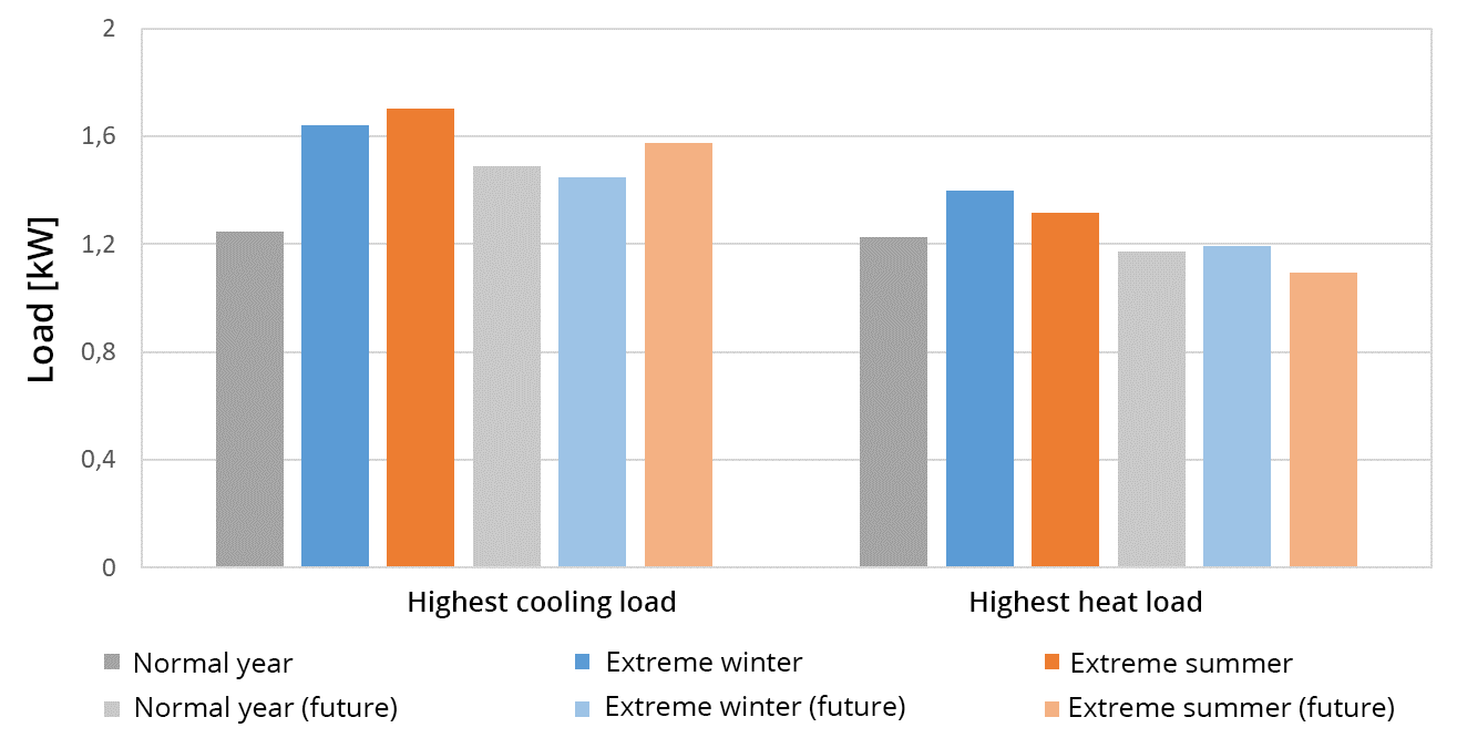
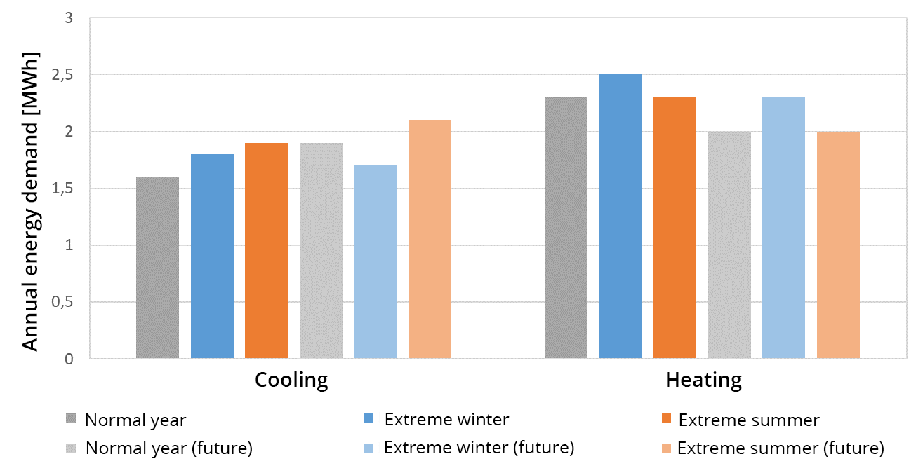
Fig. 8 and Fig. 9 show the loads and annual energy demands for heating and cooling for the six TRY data. Contrary to what could be expected at first, the highest cooling load is required in the current extreme summer and not in the extreme summer of the future forecast. Also, the cooling load of the extreme winter is also higher than the cooling load of the normal year. The annual energy demand for cooling is again in line with the expectation that during the extreme summer the most energy is required for cooling. During the normal year, both the cooling load and the energy demand for cooling increase from the current data to the future forecast. The results for heating are also in line with expectations that heating loads and energy demand are lower in the future projections than in the current TRY. Furthermore, it is noticeable that the current normal year delivers similarly comparable results, just like the future extreme winter.
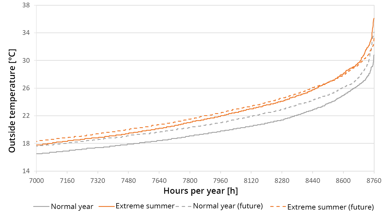
The results described can be explained by a closer look at the temperatures of the TRY. The individual hours of the year are sorted in ascending order according to temperature. This doesn’t lead to a chronological representation, but the first value corresponds to the lowest temperature and the last hour to the highest value of the corresponding TRY. Fig. 10 shows the warmest hours of the year. The maximum temperatures in the current extreme summer are higher than in the values from the future forecast, which can justify the higher cooling load. During most of the time, the temperatures of the future forecast are higher than for the current extreme summer, resulting in the higher annual energy demand for cooling. For the normal year, the future forecast is about 1.5 K higher than for the current normal year, without the temperature curves intersecting.
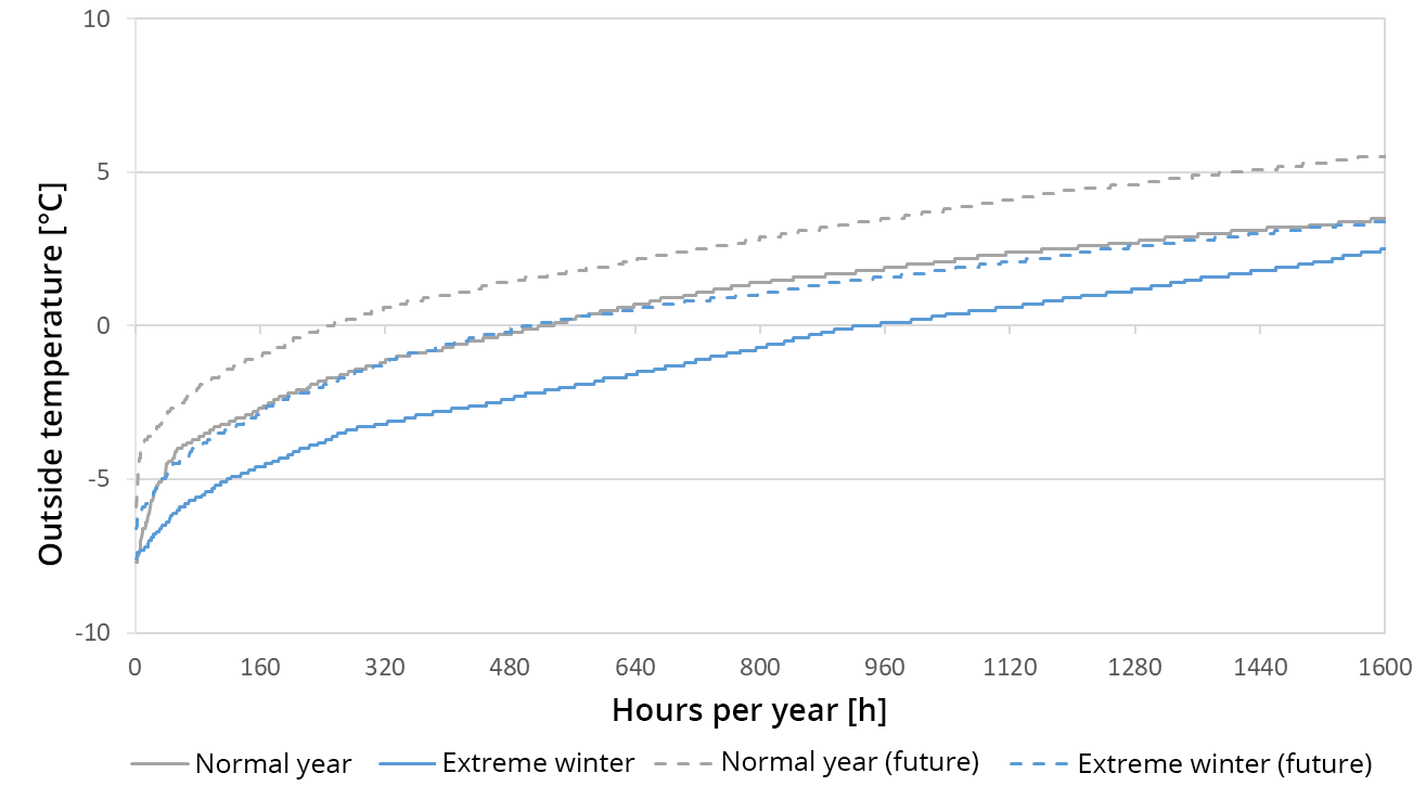
When considering the lowest temperatures during the year, the temperatures of the current normal year and the future extreme winter are almost the same (see Fig. 11), which also explains the comparable results of the heat load and the energy demand for heating. For both the future forecasts and the current TRY, the lowest temperatures are in the same range, at about -7 °C. The number of hours with negative outside temperatures in the future normal year only amount to about a quarter of the 960 hours of the current extreme winter. From comparable lowest outside temperature at the large differences in the number of more negative outside temperatures, we can derive that the differences between the maximum heat load between TRY are smaller than in the annual energy demand for heating.
Summary
The considerations of the operating mode, the control concepts and the different test reference years show the differences in the results and their cause between a cooling load calculation and an annual simulation. The defined heat period for the cooling load calculation ends with the design day and for the annual simulation a whole year is calculated. Different results are already obtained due to the different weather data in the time periods considered. The comparisons of the calculated cooling load and the highest cooling capacity in the annual simulation show that the annual simulation in the example results in slightly higher capacities throughout. However, the differences are small and are below 6% for all observations except for the “11h operation” of the cooling system. A much larger influence come from the choice of different system operating modes, such as the settings for the control concept.
From all considerations in this article, it should also be emphasized that when comparing different system concepts, not only the maximum cooling capacity should be taken into account, but also the annual energy demand. A higher cooling load does not directly correspond to a higher annual energy demand.
Since the results from the annual simulation provide even more information that can be used for a good design of the building systems - without increasing the effort for input of data - the annual simulation should be used additionally, especially when comparing different system concepts.
This article on the use of annual simulations marks the end of the article series on cooling load calculation for the time being. Starting with the development of the cooling load calculation from the tabular method of the 1970s to the current dynamic model, via a more detailed analysis of the influence of the inputs for the internal and external loads, the articles have hopefully contributed to a better assessment of the influence of the boundary conditions and input data on the results of a cooling load calculation and to a better plausibility check of the results themselves.
If the previous articles from this series are no longer available to you, you can find them at any time here: Cooling load calculation part 3